
Explainable AI: Occlusion Maps Step-by-Step
Understanding Model Decisions, One Patch at a Time

Welcome to this new installment of our series on Explainable AI (XAI) in medicine. So far, we have explored Saliency Maps, CAM, and Grad-CAM. While these methods are powerful, they are “gradient-based,” meaning they require a deep dive into the mathematical inner workings (the gradients) of an AI model to function.
In this article, we shift our focus to Occlusion Maps (also known as Occlusion Sensitivity Maps). Unlike its predecessors, this is a perturbation-based method. It doesn’t care about the internal calculus of the model; instead, it asks a very simple, clinical question: “If I hide this specific part of the image, does the model’s diagnosis change?”
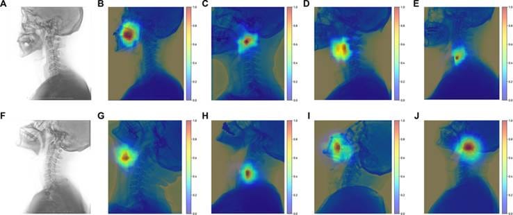
Figure : Examples of the occlusion sensitivity map for Laryngoscopy classification tasks [1]
What are Occlusion Maps?
Occlusion refers to the act of blocking or covering something. In the context of AI, an Occlusion Map is a technique used to visualize which areas of an image are most influential by systematically masking and observing the impact on the model’s output.
The most significant advantage of this method is that it is model-agnostic. Because it only looks at the input (the image) and the output (the prediction score), it can be used on any computer vision model, regardless of its architecture. All that is required is the ability to query the model—to send it an image and receive a confidence score in return. The model itself can remain entirely closed, proprietary, or remote. It is treated as a pure black box, tested through trial and error rather than inspected from within.
The Computation Process: Step-by-Step concept
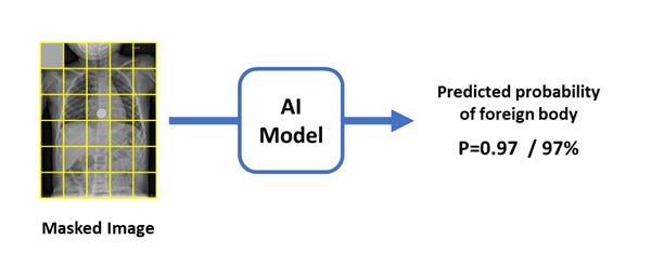
To understand how a heatmap is generated through occlusion, let’s walk through the process using the example of an X-ray being screened for foreign object detection. In this case, the AI model returns a confidence score —a score close to 1 indicating high confidence that a foreign object is present, and a score close to 0 indicating the contrary
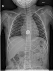
Step 0: The Baseline Reading
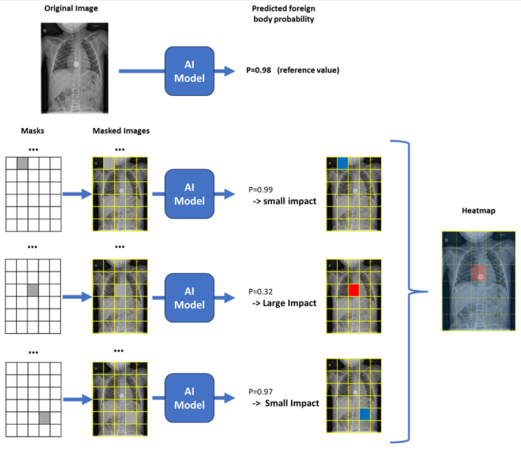
Before any occlusion happens, the algorithm needs something to compare against. The original, untouched X-ray is run through the model exactly as it is, and the resulting confidence score for the target class is recorded. This becomes the reference value against which every occluded version of the image will later be measured.
For instance, the model looks at the full X-ray and returns a 98% confidence score for “Foreign Object Detected.”
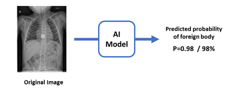
Step 1: Applying the Mask
The algorithm places a mask over the entire X-ray. This mask is mostly transparent, except for a single square patch of a specific size (e.g., 15x15 pixels) filled with a neutral color—usually gray, black, or a blurred version of the original image—to hide the underlying data at that location, typically the top-left corner by convention.
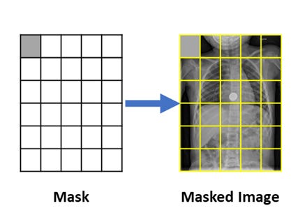
Step 2: The occluded probability
The AI model processes the image with the mask in its current position. We record the probability score for the target class.
Step 3: Calculating the Drop
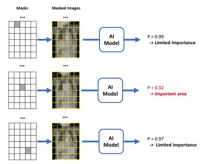
At this position, we now have two probability scores: the baseline confidence from the original image, and the confidence with the current patch masked. The difference between them tells us how important that masked region is:
Importance = Original Probability − Occluded Probability
If the confidence drops from 98% to 20% when an area is masked, we know that area was critical for the model’s decision. Conversely, if the confidence only drops from 98% to 97% when another area is masked, that region had virtually no influence on the prediction—the model barely noticed it was hidden.
Step 4: Sliding Across the Image
The patch is then moved across the image, stride by stride, systematically covering every region of the X-ray. At each new location, the patch moves just enough to cover a neighboring, previously unseen area. The same masking, measuring, and calculating steps are then repeated, producing a new importance value each time. By the end of this process, every region of the X-ray has an associated importance value, showing how much the model’s confidence dropped when that specific area was hidden.
Step 5: Generating the Heatmap
These “probability drops” are mapped onto a 2D grid. Areas where the confidence dropped significantly are colored in “hot” colors (red/orange), while areas that had no impact are “cool” (blue). The result is an Occlusion Map that can be overlaid on the original X-ray.
Healthcare Applications
In a clinical setting, Occlusion Maps offer a “sanity check” that is easy to interpret.
Feature Localization:
For classification tasks:
As an example, in Histopathology, occlusion sensitivity maps can help pathologists verify if a model is identifying specific malignant cell structures or if it is incorrectly relying on the surrounding healthy stroma.
This principle extends to any medical imaging modality and condition, allowing clinicians to verify that the model is focusing on the relevant pathological features rather than incidental findings.
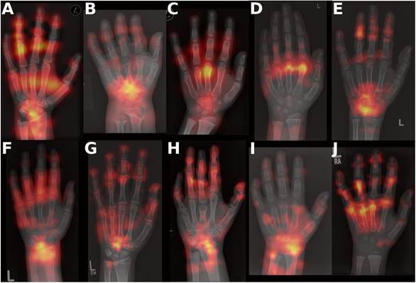
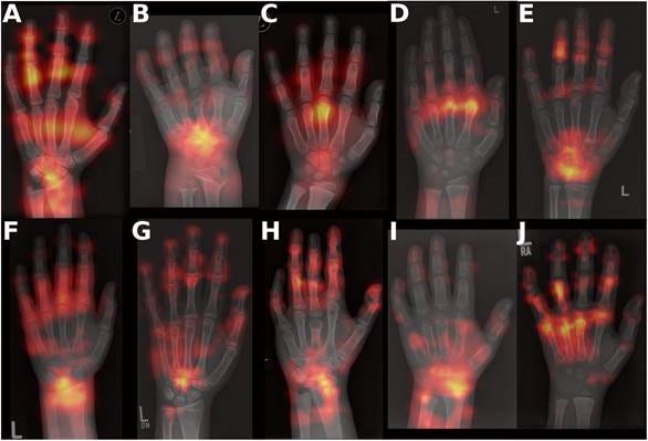
Occlusion Sensitivity Maps of sample radiographs of ten rare bone diseases: A: Hypophosphatemic rickets, X-linked dominant (XLH), B: Achondroplasia (ACH), C: Hypochondroplasia (HCH), D: ACAN-related short stature (ACAN), E: Noonan syndrome (Noonan), F: SHOX-related short stature (SHOX), G: Turner syndrome (Turner), H: Pseudohypoparathyroidism (PHP), I: Lysosomal Storage Disease (LSD), J: Silver-Russel syndrome (SRS). [3] For Image Segmentation :
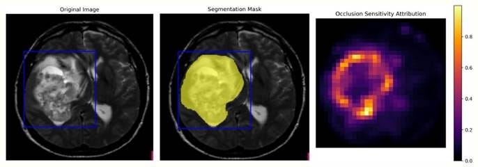
In segmentation tasks, occlusion maps can verify that the model is delineating structures for the right reasons. The heatmap highlights which regions of the image were most critical to producing the segmentation mask
Safety & Bias Detection: AI models are notorious for “cheating.” A model trained on X-rays might achieve high accuracy by looking at hospital-specific metal tags or the type of imaging equipment used, rather than the patient’s anatomy. Occlusion Maps reveal this instantly: if the heatmap glows red over a “Portable” equipment tag instead of the lungs, the model is unsafe for clinical use.
Model Comparison: Researchers can use occlusion maps to compare how a “Generalist” model versus a “Specialist” model views the same pathology, identifying which architecture is more sensitive to subtle anatomical markers.
Pros and Cons
Like any diagnostic tool, Occlusion Maps have strengths and limitations.
The Pros:
Intuitive Logic: The “What if?” approach mirrors clinical reasoning.
Model Agnostic: Works on any model, even if the internal code is inaccessible.
High Precision: If you use a very small sliding window, you can pinpoint the exact boundaries of a lesion.
The Cons:
Computationally Expensive: Because the model must re-run the image hundreds or thousands of times (once for every window position), it is much slower than Grad-CAM.
Sensitivity to Hyperparameters: The resulting map changes significantly depending on the window size and the filler color (using a black box vs. a gray box can yield different results).
Context Loss: If the window is too large, it might cover multiple features at once, making the map blurry and hard to interpret.
Edge Effect: Standard occlusion introduces sharp, artificial boundaries and “filler” colors (like solid black) that never occur in a human body. These unnatural edges can cause the confidence score to drop simply because the image looks corrupted or “out-of-distribution,” rather than because the obscured anatomy was actually relevant to the diagnosis.
“blind” sliding window: While the classic sliding window is simple, it is a “blind” geometric tool that lacks semantic or clinical awareness, and it often breaks apart anatomical structures in ways that don’t make clinical sense.
Alternative and Extensions :
A. Perturbation based methods
These approaches share the same core principle as occlusion maps—probing the model by modifying its input—but refine how the masking or sampling is performed.
Overlapping strides: “Instead of moving the patch by its full size at each step, overlapping strides move it by a smaller increment, meaning a single pixel can be occluded by multiple patch positions. This produces a more granular and precise importance map, and the final importance value for each pixel is computed by averaging the drops recorded across all positions where that pixel was covered.
Inpainting (instead of masking): “Instead of filling the occluded region with a neutral color, inpainting replaces it with a plausible reconstruction generated from the surrounding pixel context, making the masked area visually seamless. This approach aims to avoid introducing artificial color artifacts that could influence the model’s output for reasons unrelated to the occluded content, producing a more faithful importance map. [5]
Image-aware masking
Anatomical/Segment-based Masking: Instead of using a fixed square patch, anatomical or segment-based masking occludes clinically meaningful regions at once—such as a specific organ, lobe, or lesion area. This approach produces importance values that are directly interpretable by clinicians, as each value is assigned to a whole anatomical structure rather than an arbitrary grid position.
Superpixel-based Masking (LIME): Instead of a fixed square patch, superpixel-based masking groups pixels into perceptually coherent regions—called superpixels—based on local color and texture similarity, and occludes these regions as a whole. Various algorithms can be used to define these superpixels, such as QuickShift, Felzenszwalb, or SLIC, each producing slightly different region boundaries but all ensuring that the masked areas are more visually meaningful than an arbitrary grid patch. [4]
Randomized Input Sampling for Explanation (RISE ): Instead of systematically sliding a patch across the image, Randomized Input Sampling for Explanation (RISE) generates a large number of random binary masks, each randomly occluding different regions of the image at once. The model’s confidence is recorded for each masked version, and the final importance value for each pixel is computed as a weighted average of these outputs across all masks—pixels that, when visible, consistently produced high confidence scores receive a higher importance value. [4]
B. Beyond Perturbation-based Methods
Unlike perturbation-based methods, these techniques do not modify the input image. Instead, they look inside the model itself, using its internal gradients or activations to identify influential regions—making them faster but dependent on access to the model’s internal architecture.
Attention Mapping
Conclusion
Occlusion Maps provide a “brute force” but highly transparent layer of explainability. By systematically dismantling the input image, we force the AI to reveal its dependencies. For the clinician, this provides a vital layer of trust: knowing not just what the AI decided, but exactly which anatomical region held the most weight.
While Occlusion is computationally heavy, its ability to analyze a model without needing “backpropagation” makes it a versatile tool in the XAI toolkit.
References
[1] Wang M, Jia F, Yang C, et al. Identification of Difficult Laryngoscopy via Double-Pose Feature Clustering Network in Patients with Cervical Spondylosis. Intelligent Computing. 2026;5. doi:https://doi.org/10.34133/icomputing.0321
[2] Thibodeau R. Ingested foreign body. Radiopaediaorg. Published online September 1, 2023. doi:https://doi.org/10.53347/rid-174022
[3] Bolmer E, Schmidt P, Fischer I, et al. Bone2Gene: Next-generation Phenotyping of Rare Bone Diseases. Published online March 27, 2026. doi:https://doi.org/10.64898/2026.03.25.26349289
[4] Alzubaidi T, Ammar S, Alsharqi M, Rekik I, Behzad M. XAI-CLIP: ROI-Guided Perturbation Framework for Explainable Medical Image Segmentation in Multimodal Vision-Language Models. Arxiv.org. Published 2021. Accessed June 24, 2026. https://arxiv.org/html/2602.07017v1
[5] Chang CH, Creager E, Goldenberg A, Duvenaud D. Explaining Image Classifiers by Counterfactual Generation. arXiv.org. Published 2018. Accessed June 24, 2026. https://arxiv.org/abs/1807.08024